Posts Tagged ArtDiffusor
Similar, yet different: Quadratic vs. Itself?
Posted by Acoustics First in Diffusion, Product Applications, Products on July 6, 2023
For this installment of “Similar, yet different,” we will take a classic welled-quadratic sound diffuser, The Model Q, and compare its performance to itself – only installed backwards!

Taking “similar” to the extreme in this case, we are testing the difference in performance of a 1-dimensional, welled-quadratic diffuser installed in the standard welled configuration, and then installed reversed – with the sound impeding on the back side of the wells. For a bit of history, the Classic Quadratic Diffuser (or Schroeder diffuser) was designed with a grid separating the reflectors – creating wells of different depths proportional to the remainders of n2 (mod N). This design has some interesting facets.
- They are inherently symmetric if left in the original sequence.
- They are periodic (i.e. they repeat.)
- The discrete Fourier transform of the exponentiated sequence has constant magnitude.
The design principal is simple if you tear apart the math, and it’s simply wells that have a different effect on different frequencies, depending on the geometry of the wells. The Model Q is an advanced 1D-Quadratic with angled well-bottoms, which assist in smoothing out the performance and widening the 1D polar radiation. So if this design is relying on the wells to be effective, why would we reverse it?
An acoustically diffuse environment develops due to many factors, and while the frequency focus of the wells is useful, there are other scenarios where different methods may be preferred. If the geometry of the elements were flipped around, you would get the same (albeit reversed) ratio of distance, but you lose the containment and channeling that the wells provide. This imparts a diffraction on the unrestrained elements. This also allows for a different interaction between the elements, as the face of the unit is no longer planar.
Let’s look at the effect this has on the performance of the device at some different frequencies – starting low and moving up…
First, we will look at the 1150Hz performance of the devices… standard welled-install on the left, reversed on the right.

At 1150Hz, there is a little variation in the performance. Both are front focused, with a strong 1D horizontal polar response, but they are not identical. The welled-design (left) shows a broad frontal response, while the reversed design has a smoother vertical response, sharper front lobes, and stronger side performance. Overall, this difference is relatively small at this frequency.
Now, we will look at 2300Hz.

Again, we have two similar looking balloons, but there seems to be a bit more variation. The welled-design (left) shows a smoother 1D pattern in the front as the wells release sound within the same plane – at the front face of the wells. On the right you will notice sharper and more discreet lobes, but you will also notice that it has wider horizontal performance again, as it isn’t as front focused due to its free standing elements. The vertical performance is also a bit different – the welled design is broad and smoother vertically, while the reversed installation shows sharp lobes again.
Step up to 2800Hz, and we see some more drastic differences.
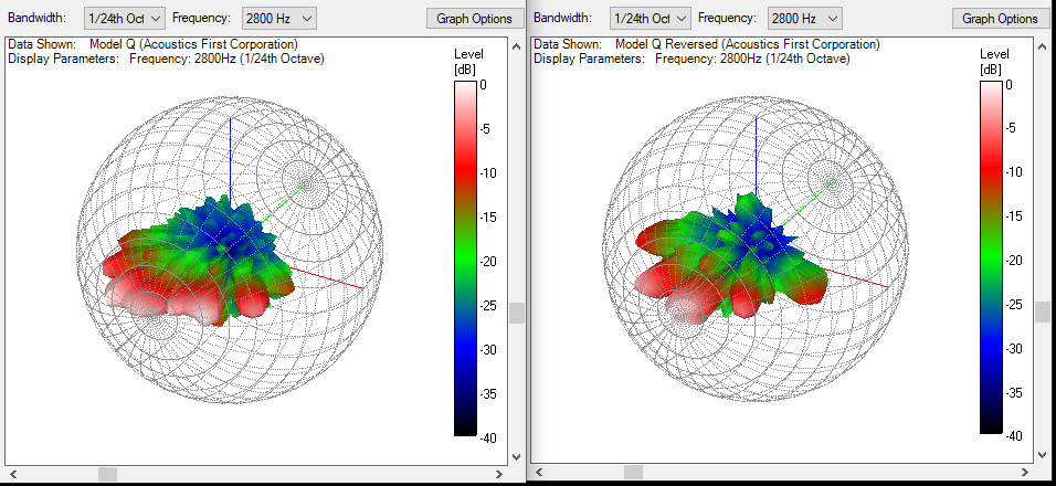
The performance of the standard welled-install (left) stays smooth and front-focused, while the lobes of the reversed install (right) have become even more distinct. Interestingly, the side lobes are even larger, showing an even wider polar pattern than before. These two instances show a marked difference between the smooth front-focused wells and the wide sharp scattering of the unrestrained elements. These two configurations are both very different, but are still both very effective at helping to disperse the incoming energy. Remember that the room develops diffusion through sound travelling in many different directions – these are not simple reflectors sending the specular energy in a single direction.
Now at 3650Hz we see a shift toward the reverse installation.
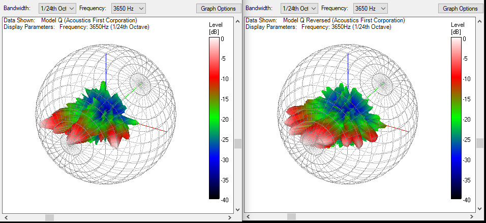
At around 4K the welled-installation (left) begins to move back front and center. It’s primary method of diffusion uses the wells to channel the energy, and at higher frequencies sound becomes much more directional. This directionality is used to create a temporal shift in the sound, as the reflections will occur out of phase from the source, and controlling that reflection is paramount to tuning this method of diffusion. However, as stated before, there are other mechanisms contribute to diffusion. The unrestrained elements on the right balloon, have hit their stride and still maintain a wide 1D polar pattern. The lobes are still sharp, showing the interaction of the elements with sound. This installation is showing the strength of its spatial dispersion, which will send acoustic energy in more directions and use the travel through the space to create a diffuse environment. It loses some of the frequency tuning of the wells, but makes up for it in the wide polar pattern.
Now for the super high frequencies – we jump straight to 10Khz.
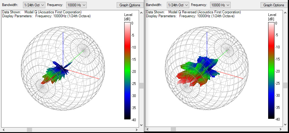
This final set shows two diffusers pushed to the limits. The welled-installation (left) is a very narrow focused beam now. You will note that it has some variance due to the interactions with the walls of the wells but all of its work is done through phase shifting at this point. In contrast, the exposed elements (right) are still allowing for a bit of diffraction to occur, and the angled faces are still allowing for a bit of spatial redirection. Also note that these polar patterns were generated with a sound source directly in front of the device at 0° incidence, and the exposed elements would offer more exposure to its surface area than a welled design at wider angles of incidence.
In summary…
Diffusion develops using many different variables, including the untreated walls of the space. While both of these installations are functioning in nearly identical frequency ranges due to their geometry, the mechanisms which they work are slightly different and have different strengths. The welled-design (in classic temporal Schroeder configuration) uses the wells to channel sound and address the frequencies in a tuned and controlled fashion. By simply flipping the device around, however, you change its performance from a controlled time shift, to an unrestrained spatial redirector, which imparts time shift through dispersion, diffraction, and distance travelled – further reducing intensity by having a wide 1D diffusion polar pattern. Both have scenarios which one configuration would be preferable over the other, making the Model Q diffuser a very versatile device.
Both configurations are literally two sides of the same coin… they work in different ways, over the same frequencies, providing results – no matter how you flip them.
ArtDiffusor® Model D vs. Aeolian®: Similar, yet different.
Posted by Acoustics First in Diffusion, Product Applications, Products, Uncategorized on November 12, 2020

Today on, “Similar, yet different…” we are going to analyze two more of our acoustic diffusers and compare/contrast their designs and functionality… and this one is a doozy; The Model D vs. The Aeolian®. These two diffusers have some very interesting similarities and some surprising differences – so lets get started!
We have discussed the Aeolian® construction before, so we will start here with a quick recap as a reference point. The Aeolian® started life as a blocky-looking diffuser – just like the Model C, but the implementation is different. While the Model C retains its “blocky” appearance, the Aeolian® has run through a mathematical process called “bicubic interpolation.” This smooths the transition from one block to the next, creating the wavy appearance of the Aeolian® diffuser.
So, keep that in mind: The diffuser was tuned with different height blocks and then the transitions were smoothed.

Look at the smooth curves of the Aeolian®.
The Art Diffusor® Model D has multiple layers of math below its curved surface. While the Aeolian® started life as “Blocks” of different heights… the Model D started life as “Rings” of different sizes and heights. The calculation for the heights is identical to the mathematics used in tuning the Aeolian®, but why different sized rings?
There is an older diffuser design known as a Maximum Length Sequence (MLS) diffuser. These were tuned to different frequencies using a specific depth, and different spacings of “lands and valleys.”
MLS Diffusers had same depth wells of different sizes and spacings…
The Model D started with the concept of twisting the MLS spacings into rings, and changing the size of the rings. Then to break the “MLS mold” of having the same depth, this MLS ring structure is raised to different heights using Quadratic Residue calculations… effectively combining the rings of MLS spacings with different QRD heights. While this could have been where this stopped, we wanted to interject more randomness into the equation.
Wherever the rings of different heights intersected, we decided to change the heights by values relative to the difference between the two rings. This height variation is what is responsible for the “random” waviness. This was accomplished with different Boolean Functions, to either add or subtract height where the rings intersected.

You can really see the variation in the geometry of the Model D… look at the ripples in the rings.
This method of using Boolean Functions inserts a known-height randomization into a hybrid MLS/Quadratic system. (That’s a mouthful.) The final step, after refining the ring size, height, position and intersection parameters… was to smooth the whole geometry with “Bicubic Interpolation.” That’s right. This final step smooths all the transitions from the heights, just like the blocks of the Aeolian®.
So onto the Simple Similarities!
Both diffusers use a quadratic residue calculations to get the main heights of the diffusive elements. Both diffusers are finished off with a helping of “Bicubic Interpolation” to smooth it all out. This gives them both a very organic look… The Aeolian® looks a bit like rolling waves, and the Model D resembles droplets of rain in a puddle…
They do perform quite a bit differently though.
The Aeolian® has great lower mid-band performance… while the Model D is a beast in the upper mid-bands starting about 2.5K. The difference is in the severity of the geometry. The Aeolian® is a gently rolling surface which redirects the waveforms uniformly through a wide range of frequencies. The Model D has a very irregular surface. With the different ring sizes, heights, locations and boolean functions… it’s meant to target and shred mid to high frequencies. Both diffusers are asymmetric – and affect different frequencies in different ways.
The Aeolian® is also deeper than the Model D – and this depth is a single resonant cavity… allowing it to be a great bass absorber as well. The Model D is useful in environments where you have bass control in place, but really need to diffuse the upper mid range and bring those frequencies to life… or maybe shred some flutter echos or comb filtering. There are scenarios where both are used in the same environment – but for different reasons.
In Conclusion...
While both the ArtDiffusor® Model D and the Aeolian® both look like liquids frozen in time, they have some other similarities in the math behind them… Yet they are still as different as rolling waves versus droplets of rain in a puddle.
ArtDiffusor® Model C vs. Aeolian®: Similar, yet different.
Posted by Acoustics First in Diffusion, Product Applications, Products, Uncategorized on September 24, 2020

For this installment of “Similar, yet different” we look at The ArtDiffuser® Model C and the Aeolian® Sound Diffuser.
While these two diffusers look very different, there are a fair amount of similarities between them. Their physical size and depth allow them both to be great mid-frequency diffusers, but did you know that the Aeolian® started life as a blocky-looking diffuser – just like the Model C? It’s true!

ArtDiffusor® Model C array on a hanging bass trap.
The mathematics behind the two diffusers is similar, but the implementation is different. While the Model C retains its “blocky” appearance, the Aeolian has run through a mathematical process called “bicubic interpolation.” Without turning this into a math-heavy post, if you take a “blocky” design like the Model C and run its geometry through bicubic interpolation, you get a “curvy” surface like the Aeolian® – It “smooths” the transition from one block to the next in a 3 dimensional matrix.
While they did not begin as identical geometries, they were similar in their height ratios – with the Aeolian® starting with fewer blocks in a more random distribution, and a slightly taller maximum height. They both effect similar frequency ranges, with the Aeolian® going slightly lower and higher due to its depth and interpolated surface. The pattern and type of the diffusion is also different because of the different geometries – the Model C has blocks, and the edges of those blocks introduce a great deal of edge “diffraction” – which is what happens when a wave interacts with an edge, or corner, of a surface. It bends and shears around the edge, which helps break up the continuity of the waveform, where the Aeolian® takes the approach of redirecting most of the energy off a randomized and continually-curved surface.
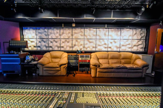
Aeolian® Diffuser array on the back wall of Big3 Studios.
It is important to note that the two are similar, yet different in their absorption numbers as well. With the Aeolian® being deeper with a single large cavity, it provides a bit more absorption in the low frequencies than the Model C, which is a more rigid geometry containing smaller elements. Depending on the space, this may be a useful addition to the diffusive properties. While some spaces need the extra absorption, some are pretty well balanced already and are just looking to “sweeten” the sound a bit.
On the surface, they are both a nominal 2’x2′ square of thermoformed Class A plastic with lightly textured surface. That is the extent of the visual similarities, and we cannot hide the aesthetic differences between the two devices. The ArtDiffusor® Model C is a “classic” diffuser. Many have been looking at these for the better part of 3 decades now. It’s a classic design at this point with no need for introduction – it is what the quintessential diffuser “looks” like. In fact, when many people think of a diffuser – the Model C is what they visualize! The Aeolian® is a modern rendition of the classic design. Using modern calculation techniques, we can now present the type of diffusion the Model C is famous for, in a different way.
While the two geometries look entirely different, and perform a bit differently, they have a common heritage as mathematical, 2-dimensional diffusers. You could say that the Model C is the grandparent of the Aeolian®, and that pedigree has been passed on – having a similar foundation, but a different final interpretation.
Art Diffusor® Nouveau™ – Limitless possibilities.
Posted by Acoustics First in Diffusion, Product Applications, Products, Uncategorized on June 5, 2020

ArtDiffusor® Nouveau™ on a wall with a dark stain – framed.
Hey! Here’s another installation of our new ArtDiffusor® Nouveau™. For this install, these four boards were not only stained, but also framed out to enhance the design aesthetic. From different paints and stains, to mounting techniques, there are limitless possibilities for customization to create your own unique and functional sound diffusing arrays.
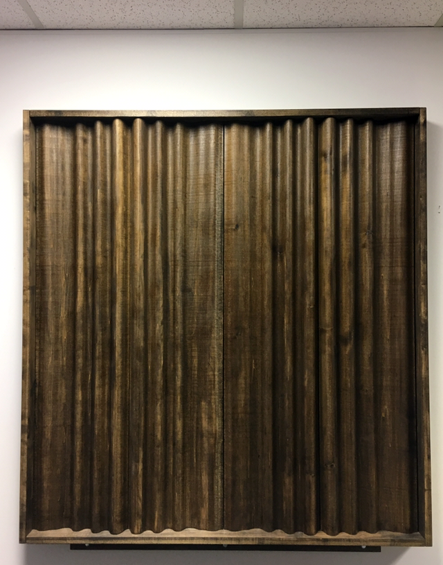
ArtDiffusor® Nouveau™ on a wall with a dark stain – framed.
Big3 Studios – Aeolian® Diffusers
Posted by Acoustics First in Diffusion, Product Applications, Products, Recording Facilities, Studio Control Room, Uncategorized on August 17, 2018

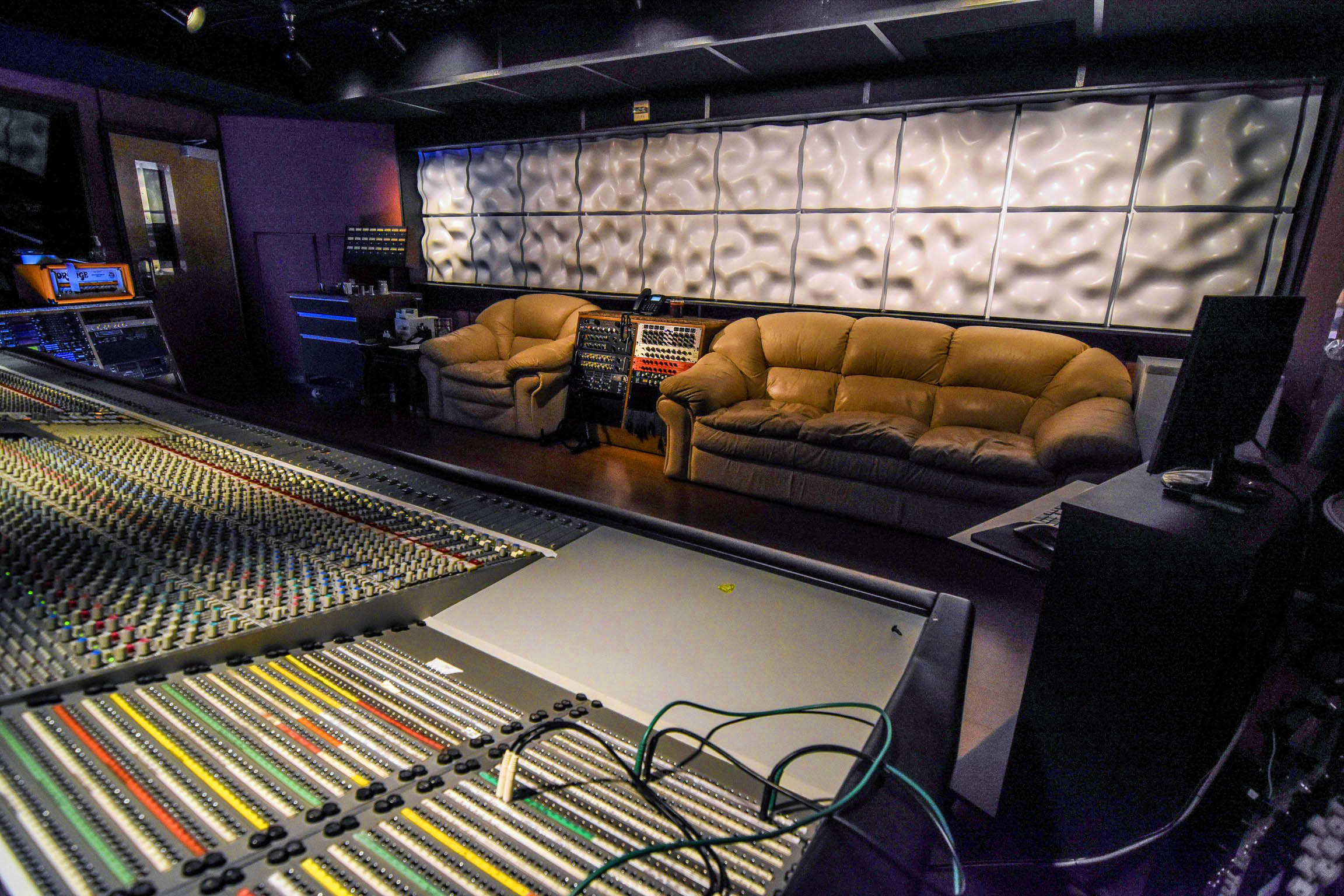
Aeolian® Diffusers in Big3 Studios
We recently received these wonderful installation pics from our friends at Big3 Studios in Florida. They redid the back wall in one of their control rooms using our Aeolian® Sound Diffusers. In a couple of the pics you can also see our Model C & Model F Art Diffusors® (black) in the ceiling!


You must be logged in to post a comment.